Fraunhofer Diffraction and the 2D Fourier Transform; Solving the Heat/Diffusion Equation with Fourier Series
Contents
Fraunhofer Diffraction and the 2D Fourier Transform
Reference:
https://en.wikipedia.org/wiki/Fraunhofer_diffraction_%28mathematics%29
The complex amplitude of a diffracted wave far from an aperture can be calculated using the Fraunhofer diffraction integral:
 are the coordinates across the aperture,
  is the complex amplitude across the aperture, and
  are the coordinates at the screen. The complex amplitude at each position
  can be seen as the 2D Fourier coefficient calculated for the frequency
  .
.
The 2D Fourier transform
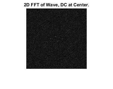
The two dimensional fourier transform is computed using 'fft2'. Let's try a simple example to demonstrate the 2D FT.
lambda=10;  %Try adjusting and look at the result.
k=2*pi/lambda;
[X,Y]=meshgrid(1:200,1:200);
kx=k*.2;
ky=k*.4;

Wave1=real(exp(i*k*X));
Wave2=real(exp(i*(kx*X+ky*Y)));
%Wave=ones(size(X));
Wave=Wave1+Wave2;
Noise=10*randn(size(Wave));
Wave=Wave+Noise;
figure;imshow(Wave,[]);title('Wave')

F_Wave=fft2(Wave);
figure;imshow(abs(F_Wave),[]);title('2D FFT of Wave')
F_Wave_Shift=fftshift(F_Wave);
figure;imshow(abs(F_Wave_Shift),[]);title('2D FFT of Wave, DC at Center.')
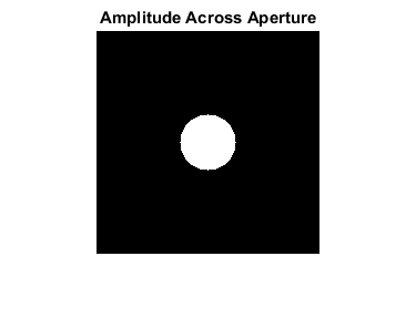
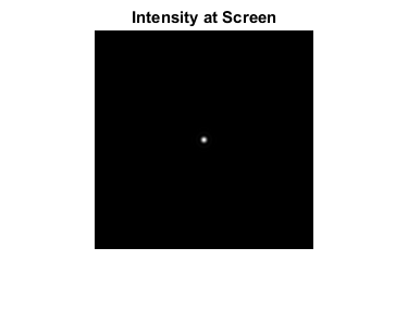
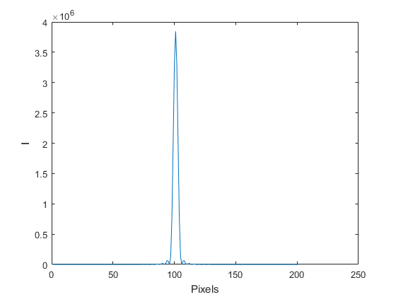
The Circular Aperture
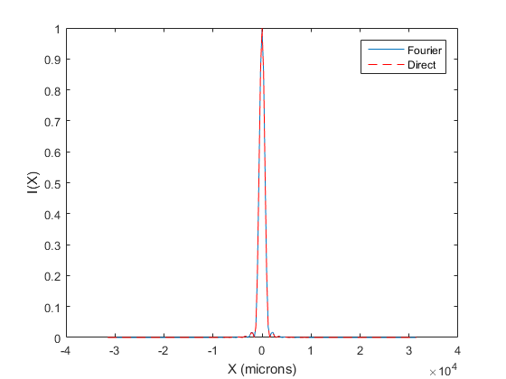
Let's revisit diffraction from a circular aperture.
Lambda=.633;        %Wavelength of laser (micron)
D=50;               %Diameter of aperture (micron)
Z_Meters=.1;        %Screen distance in meters
Z=Z_Meters*10^6;    %Screen distance in microns

MeshSpacing=1;      %Sampling across aperture (micron)
MeshSize=200;       %Size of Screen (micron)

%Calculate and show the Amplitude across the aperture.
[XGrid,YGrid]=meshgrid((-MeshSize/2:MeshSpacing:MeshSize/2),(-MeshSize/2:MeshSpacing:MeshSize/2));
R=sqrt(XGrid.^2+YGrid.^2);
A=R<=D/2;  %The Amplitude across aperture (plane wave has constant amplitude, phase)
figure;imshow(A);title('Amplitude Across Aperture')

%Do the the 2D fft and show the result.
U=fftshift(fft2(A));
I=abs(U).^2;
figure;imshow(I,[]);title('Intensity at Screen')
figure;imshow(log(I),[]);title('Log Intensity at Screen')
figure;plot(I(101,:));xlabel('Pixels');ylabel('I')

% Now let's figure out the spacing of the pixels in I.
% The spacing of frequencies in the Fourier transform is 1/L
SZ=size(A,1);
FrequencySampling=1/(SZ*MeshSpacing); %units of 1/microns
[FGridX,FGridY]=meshgrid((0:SZ-1),(0:SZ-1));
FGridX_Shift=fftshift(FGridX);
FGridX_Shift(FGridX_Shift>SZ/2)=FGridX_Shift(FGridX_Shift>SZ/2)-SZ;
FGridY_Shift=fftshift(FGridY);
FGridY_Shift(FGridY_Shift>SZ/2)=FGridY_Shift(FGridY_Shift>SZ/2)-SZ;

FX=FGridX_Shift*FrequencySampling;
FY=FGridY_Shift*FrequencySampling;
X=FX*Lambda*Z;
Y=FY*Lambda*Z;

% Plot with units
I_norm=I/max(I(:));
X_center=X(101,:)+eps;
figure
plot(X_center,I_norm(101,:));xlabel('X (microns)');ylabel('I(X)')

% Compare to Airy disc
k=2*pi/Lambda;
a=D/2;
SinTheta=X_center./sqrt(X_center.^2+Z.^2);
I_Airy=(besselj(1,k*a*SinTheta)./(k*a*SinTheta)).^2;
I_Airy_norm=I_Airy/max(I_Airy(:));

hold on
plot(X_center,I_Airy_norm,'r--')
legend('Fourier','Direct')

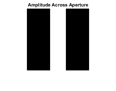
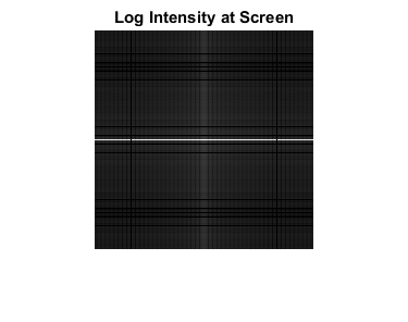
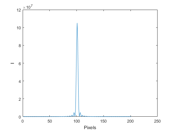
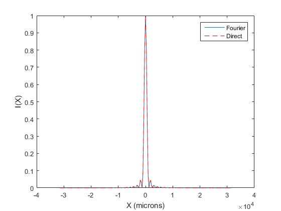
The Finite-Width Single Slit
lambda=.633;        %Wavelength of laser (micron)
a=50;               %Diameter of aperture (micron)
Z_Meters=.1;        %Screen distance in meters
Z=Z_Meters*10^6;    %Screen distance in microns

MeshSpacing=1;  %Sampling across aperture (micron)
MeshSize=200;
[XGrid,YGrid]=meshgrid((-MeshSize/2:MeshSpacing:MeshSize/2),(-MeshSize/2:MeshSpacing:MeshSize/2));
R=abs(XGrid);
A=R<=(a/2);  %The Amplitude across aperture
figure;imshow(A);title('Amplitude Across Aperture')

U=fftshift(fft2(A));
I=abs(U).^2;
figure;imshow(I,[]);title('Intensity at Screen')
figure;imshow(log(I),[]);title('Log Intensity at Screen')
figure;plot(I(101,:));xlabel('Pixels');ylabel('I')

% Now let's figure out the spacing of the pixels in I.
% The spacing of frequencies in the Fourier transform is 1/L
SZ=size(A,1);
FrequencySampling=1/(SZ*MeshSpacing); %units of 1/microns
[FGridX,FGridY]=meshgrid((0:SZ-1),(0:SZ-1));
FGridX_Shift=fftshift(FGridX);
FGridX_Shift(FGridX_Shift>SZ/2)=FGridX_Shift(FGridX_Shift>SZ/2)-SZ;
FGridY_Shift=fftshift(FGridY);
FGridY_Shift(FGridY_Shift>SZ/2)=FGridY_Shift(FGridY_Shift>SZ/2)-SZ;

FX=FGridX_Shift*FrequencySampling;
FY=FGridY_Shift*FrequencySampling;
X=FX*Lambda*Z;
Y=FY*Lambda*Z;

% Plot with units
I_norm=I/max(I(:));
X_center=X(101,:)+eps;
figure
plot(X_center,I_norm(101,:));xlabel('X (microns)');ylabel('I(X)')

% Compare to Theory
k=2*pi/Lambda;
SinTheta=X_center./sqrt(X_center.^2+Z.^2);

%Theory (See also Mar_23.m)
% The FT of the 'rect' function is the 'sinc' function.
%Make our own sinc function
mysinc=@(x)sin(pi*x)./(pi*x);
SinTheta=X_center./sqrt(Z.^2+X_center.^2);
SingleSlitDif=mysinc(SinTheta/Lambda*a).^2;

hold on
plot(X_center,SingleSlitDif,'r--')
legend('Fourier','Direct')